
Sensitivity investigations of thin-walled shell structures using transient finite element analysis and finite perturbations
- contact: Prof. Dr.-Ing. Karl Schweizerhof
Dipl.-Ing. Eduard Ewert - project group: Finite Element Analyses
Description of the Project
In standard static stability investigations of structures applying the finite element method bifurcation and snap-through points usually are detected by monitoring the triangular decomposition of the stiffness matrix within the solution process. For such analyses in addition path-following procedures are used to obtain the load-deflection curves. However, the real meaning and physical realisation of these curves are often questionable, e.g. for structures with many bifurcation points and multiple branches or contact problems. Besides this many parts of the load deformation path cannot be computed due to numerical respectively convergence problems occurring with almost singular matrices. Moreover, for practical design purposes not only the equilibrium state itself is significant but also the “robustness” of such states against finite perturbations in contrast to infinitesimal perturbations which can be detained using transient analyses.
In the case of a system with many equilibrium states at a defined load level a finite perturbation can transfer the mechanical system from one stable equilibrium state to another one or in some cases even to an unbounded motion. A sensitivity measure is defined as the reciprocal value of the minimum kinetic energy, necessary for this transfer: S= 1/Wkin,min. From this definition it follows that a mechanical system is stable and insensitive for S=0. The sensitivity is increasing with the reduction of the kinetic perturbation energy. An instable system is obtained for S~0.
The following steps within a computation have to be performed for the determination of sensitivity:
- Static analysis up to the equilibrium state to be investigated
- Introduction of a kinetic perturbation energy, for example definition of velocity impulse distribution and amplitude
- Transient analysis determining the perturbed motion
- Analysis of the perturbed motion necessary to find the minimal perturbation energy
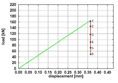
For example, the load deflection curve, shown in Fig. 1, is determined for an axially loaded cylinder. Stable equilibrium states are marked in green and unstable ones in red. It is obvious that only one stable equilibrium state exists at each load level. Further up to a load range of about 50 kN any amount of perturbation can be applied to the structure, without causing failure (elastic material behaviour assumed). The structure will vibrate around the equilibrium state. Above 50 kN two equilibrium states exist at each load level, one stable and one unstable equilibrium state. In this case the cylinder will vibrate around the equilibrium state only for sufficiently low perturbation energies. If the perturbation energy is large enough, the motion leaves the basin of attraction of the original equilibrium state and buckling is obtained (Fig. 2), which indicates a failure.If the structure is vibrating around the original equilibrium state, the perturbation energy can be increased If the structure leaves the basin of attraction of the original equilibrium state, which means, the structure moves to another stable equilibrium state or performs an unbounded motion, then the perturbation energy must be reduced
In this context the following questions are of interest:
1. Which velocity perturbation vector pattern and amplitude leads to the highest sensitivity?
2. How can the perturbed motion be analysed, in order to make efficient decisions about the kind of the motion?
 |
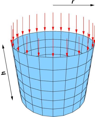 |
| Figure 1: System und load deflection curve for static loading | Figure 2: Cylinder, orbitally stable in the prebuckling range (left figure) and buckling formation after sufficiently large kinetic perturbation (right figure). |